Model evaluation¶

Evaluating an online model is fundamentally different from the batch setting. There's no fixed train/test split — data arrives one sample at a time. This recipe explains progressive validation, the standard evaluation protocol for online learning, and shows how to use River's evaluate module.

Why not train/test split?¶

In batch machine learning, you split your data into a training set and a test set. The model trains on one chunk and is evaluated on the other. This works because you have all the data upfront.

In online learning, data arrives as a stream. You don't have the luxury of holding data back. Instead, we use progressive validation (also called prequential evaluation or test-then-train):

1. A new sample x arrives
2. The model makes a prediction before seeing the answer
3. The true label y is revealed
4. The metric is updated with the prediction and the true label
5. The model learns from (x, y)

Because the model is always tested on data it hasn't trained on yet, progressive validation gives an honest estimate of real-world performance — no separate test set needed.

The manual loop¶

Let's start with the explicit loop so you can see exactly what's happening. We'll use the Phishing dataset (a binary classification task) and a logistic regression:

from river import datasets, linear_model, metrics, preprocessing

model = preprocessing.StandardScaler() | linear_model.LogisticRegression()
metric = metrics.Accuracy()

for x, y in datasets.Phishing():
    y_pred = model.predict_one(x)
    metric.update(y, y_pred)
    model.learn_one(x, y)

metric

Accuracy: 89.28%

This is the essence of progressive validation. Every sample is first used for testing, then for training.

Using evaluate.progressive_val_score¶

The loop above is so common that River provides evaluate.progressive_val_score to do it in one call. It handles the predict/update/learn cycle for you, and picks the right prediction method (predict_one vs predict_proba_one) based on the metric:

from river import evaluate

model = preprocessing.StandardScaler() | linear_model.LogisticRegression()

evaluate.progressive_val_score(
    dataset=datasets.Phishing(),
    model=model,
    metric=metrics.Accuracy(),
)

Accuracy: 89.28%

Use print_every to see progress during evaluation:

model = preprocessing.StandardScaler() | linear_model.LogisticRegression()

evaluate.progressive_val_score(
    dataset=datasets.Phishing(),
    model=model,
    metric=metrics.Accuracy(),
    print_every=250,
)

[250] Accuracy: 84.00%
[500] Accuracy: 86.80%
[750] Accuracy: 88.40%
[1,000] Accuracy: 89.10%
[1,250] Accuracy: 89.28%

Accuracy: 89.28%

Choosing metrics¶

River's metrics module has all the usual suspects. For classification: Accuracy, F1, Precision, Recall, ROCAUC, LogLoss, etc. For regression: MAE, MSE, RMSE, R2, SMAPE, etc.

When you pass a metric that compares probabilities (like ROCAUC), progressive_val_score automatically uses predict_proba_one instead of predict_one:

model = preprocessing.StandardScaler() | linear_model.LogisticRegression()

evaluate.progressive_val_score(
    dataset=datasets.Phishing(),
    model=model,
    metric=metrics.ROCAUC(),
)

ROCAUC: 95.07%

You can also combine multiple metrics with +:

model = preprocessing.StandardScaler() | linear_model.LogisticRegression()

evaluate.progressive_val_score(
    dataset=datasets.Phishing(),
    model=model,
    metric=metrics.Accuracy() + metrics.F1() + metrics.LogLoss(),
)

Accuracy: 89.28%
F1: 87.97%
LogLoss: 0.3301120464388312

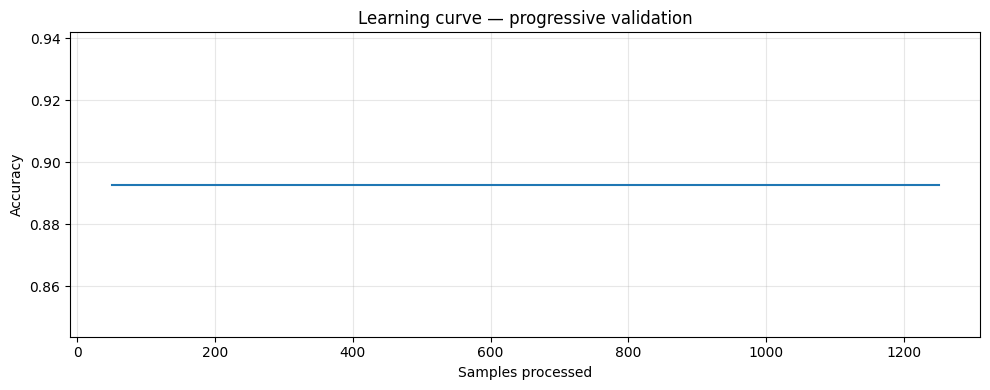
Tracking performance over time with iter_progressive_val_score¶

Often you want to see how a model's performance evolves as it processes more data. iter_progressive_val_score yields results at regular checkpoints, which you can collect and plot:

model = preprocessing.StandardScaler() | linear_model.LogisticRegression()

checkpoints = list(evaluate.iter_progressive_val_score(
    dataset=datasets.Phishing(),
    model=model,
    metric=metrics.Accuracy(),
    step=50,
))

# Each checkpoint is a dict
checkpoints[-1]

{'Accuracy': Accuracy: 89.28%, 'Step': 1250}

import matplotlib.pyplot as plt

steps = [c["Step"] for c in checkpoints]
accs = [c["Accuracy"].get() for c in checkpoints]

plt.figure(figsize=(10, 4))
plt.plot(steps, accs)
plt.xlabel("Samples processed")
plt.ylabel("Accuracy")
plt.title("Learning curve — progressive validation")
plt.grid(alpha=0.3)
plt.tight_layout()
plt.show()

Regression example¶

Progressive validation works the same way for regression. Here we predict Trump's approval rating:

from river import optim

model = (
    preprocessing.StandardScaler()
    | linear_model.LinearRegression(optimizer=optim.SGD(0.001))
)

evaluate.progressive_val_score(
    dataset=datasets.TrumpApproval(),
    model=model,
    metric=metrics.MAE(),
    print_every=200,
)

[200] MAE: 7.955145
[400] MAE: 4.738404
[600] MAE: 3.433783
[800] MAE: 2.787887
[1,000] MAE: 2.324138
[1,001] MAE: 2.321971

MAE: 2.321971

Delayed labels¶

In real-world scenarios, the ground truth often arrives with a delay. For example, a fraud detection system makes a prediction at transaction time, but the label (fraud or not) may only be confirmed days later. During that delay, the model keeps making predictions without learning from the pending labels.

progressive_val_score supports this via the moment and delay parameters. moment identifies a field in each sample that defines temporal ordering, and delay specifies how long the label takes to arrive. The delay must be compatible with the moment type — if the moment is a datetime, use a timedelta; if it's an integer (like an ordinal date), use an integer:

model = (
    preprocessing.StandardScaler()
    | linear_model.LinearRegression(optimizer=optim.SGD(0.001))
)

evaluate.progressive_val_score(
    dataset=datasets.TrumpApproval(),
    model=model,
    metric=metrics.MAE(),
    moment="ordinal_date",
    delay=1,
)

MAE: 2.321971

With a delay, the model must predict using an older version of itself — just like in production. This typically gives a more realistic (and lower) performance estimate.

Measuring time and memory¶

You can track resource usage with show_time and show_memory:

model = preprocessing.StandardScaler() | linear_model.LogisticRegression()

evaluate.progressive_val_score(
    dataset=datasets.Phishing(),
    model=model,
    metric=metrics.Accuracy(),
    print_every=500,
    show_time=True,
    show_memory=True,
)

[500] Accuracy: 86.80% – 00:00:00 – 5.88 KiB
[1,000] Accuracy: 89.10% – 00:00:00 – 5.88 KiB
[1,250] Accuracy: 89.28% – 00:00:00 – 5.88 KiB

Accuracy: 89.28%